
If Spotify raised its price by 20% tomorrow, would you keep your subscription or cancel it? Your answer is your price sensitivity, which measures how much a change in price changes a customer's willingness to buy.
To measure price sensitivity across your own customers, you run a pricing survey, and three survey types give you six different ways to read it. A Van Westendorp survey shows how wide the range of acceptable prices is, and a Gabor Granger survey shows how fast demand drops as the price goes up. A conjoint analysis survey gives you the other four reports from the same set of answers: price importance, marginal willingness to pay, rejection rate and a revenue simulator.
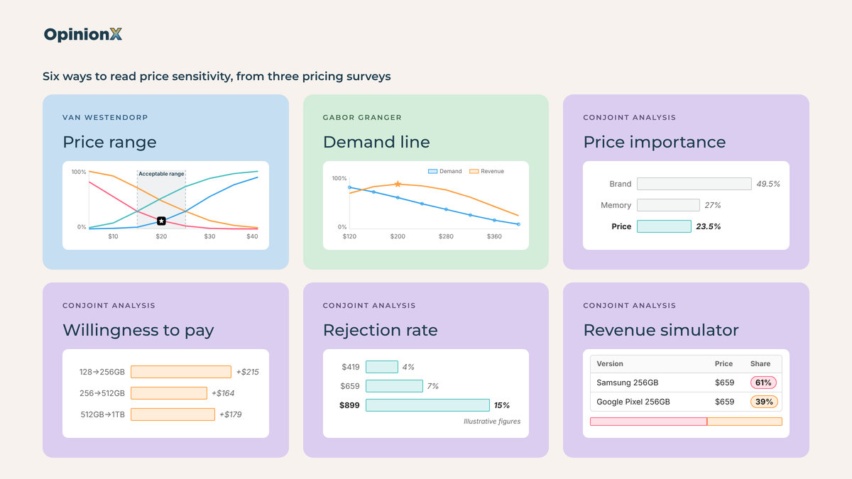
Each of the six measures a different side of price sensitivity, and the most useful finding usually comes from comparing customer segments, not from any single price result. In a conjoint survey of 1,363 people on OpinionX, price drove 25% of choices for Android owners and 21% for iPhone owners, while iPhone owners would pay about $711 more for an iPhone than a Samsung, against $208 for Android owners.
The sections below explain what price sensitivity is and how each of the six reports works with actual survey data, plus how to calculate price elasticity from survey results, how to compare price sensitivity across customer segments and which mistakes make a price sensitivity study useless.
What is price sensitivity?
Price sensitivity is how much a change in price changes the number of people willing to buy a product. Low price sensitivity means a price increase barely affects demand, generally because buyers care more about the brand, the quality or a specific feature than about the price. High price sensitivity means even a small price rise makes lots of people walk away, and those buyers will likely accept trade-offs (like a single-seat plan instead of a team account) to keep the price down.
💡 Price elasticity is how economists put a figure on price sensitivity, and you calculate it by dividing the percentage change in demand by the percentage change in price. An elasticity of −2 means a 10% price rise cuts demand by 20%, while an elasticity of −0.5 means the same rise cuts demand by only 5%. The minus sign is there because demand goes down when price goes up.
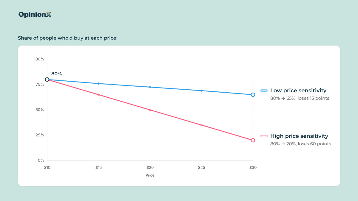
Price sensitivity isn't a fixed trait of a person, and the same person's price sensitivity changes based on:
Who's buying → A UX manager buying Figma for a team with a company budget reacts to price differently from the same person buying a design tool with their own money.
What they're buying → People accept a higher price for a sandwich in an airport than in a supermarket, because the alternatives and the context are different.
Why they're buying → A gift for someone else often gets a bigger budget than the same product bought for yourself.
Small price changes have big effects on profit, which is why price sensitivity is worth measuring. Based on the finances of 2,463 companies, Michael Marn and Robert Rosiello of McKinsey worked out that a 1% price improvement with no loss of sales volume raises operating profit by 11.1% (Harvard Business Review, 1992). The catch is the "no loss of sales volume" bit, and that's where price sensitivity research comes in: it tells you how much volume a price change would actually cost you in customer churn.
Why measure price sensitivity instead of just calculating an optimal price?
Measuring price sensitivity beats a single "optimal price" survey in a few ways:
It tells you how your customers will react to price changes you haven't made yet, which is much lower risk than measuring actual revenue changes after a price increase.
It shows which customer segments are most or least open to price changes, so you can tailor your pricing strategy to the right customers.
People state prices in surveys about 21% higher than they actually spend (Schmidt and Bijmolt, 2020), so the differences in sensitivity between groups give you more reliable data than a specific optimal price.
Product teams use price sensitivity research to make four kinds of decisions:
Prioritise the roadmap by how much customers would pay for each new feature, not only by how often they ask for it (our guide to prioritisation techniques compares the usual ways teams decide what to build).
Find the customer segments that would pay the most, meaning the groups of customers (by company size, job role or current plan) whose demand drops least as the price goes up.
Design pricing tiers by putting the features customers value most into the higher tiers.
Position the product as a budget or premium option, based on where customers think the price starts to signal low quality.
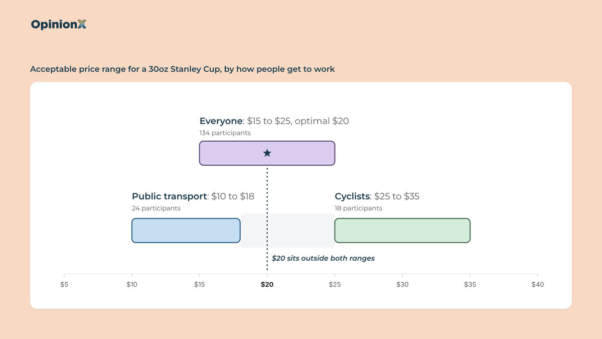
Every one of those decisions compares features, segments or tiers against each other, which is why comparing price sensitivity results tells you more than an optimal price survey ever can. A pricing survey that reports one optimal price for "everyone" also averages together customers who'd pay $10 and customers who'd pay $40, and ends up recommending a price neither group wants. The segment comparison section below shows this happening with actual survey data.
Which surveys measure price sensitivity, and what does each one show?
Three survey types measure price sensitivity: Van Westendorp, Gabor Granger and Conjoint Analysis.
Van Westendorp and Gabor Granger each give you one reading of price sensitivity, while a conjoint survey gives you four, because the same answers feed four different analyses: price importance, marginal willingness to pay, rejection rate and a revenue simulator.
The table below compares all six price sensitivity analysis methods, which survey each one comes from, what you need before you start and the pricing decision each one suits best.
| Way to measure | Survey it comes from | Price sensitivity signal | What you need first | Best for this decision | What it gives up |
|---|---|---|---|---|---|
| Acceptable price range | Van Westendorp | How wide the range of acceptable prices is, and how steeply the lines rise either side of the optimal price | A product description, no prices | Pricing a new product with no price yet | No demand or revenue figures unless you add two extra questions |
| Demand line | Gabor Granger | The share of people who'd buy at each price, which gives price elasticity between any two prices | A price range you choose before launch | Choosing the price that earns the most revenue for one product | Only tests the prices you chose, so a range that's too low hides the actual answer |
| Price importance | Conjoint analysis | The share of each choice driven by price rather than by features | Categories, options and realistic prices | Finding which customer segments care most about price | A relative figure that changes with the prices you test, so it says nothing about what to charge |
| Marginal willingness to pay | Conjoint analysis | Dollars customers would add to the price for each feature upgrade | A price category in the conjoint survey | Deciding which features go in which pricing tier | Only values the gap between two options, never the whole product |
| Rejection rate | Conjoint analysis | How often each price makes participants reject every product version shown | "None of the above" turned on before launch | Finding the price where people stop buying at all | The wording of the "None" button changes how often people press it |
| Revenue simulator | Conjoint analysis | How predicted market share and revenue change when you reprice one product version against others | A price category, ideally with "None of the above" too | Pricing against a competitor or between your own tiers | Compares the versions you build against each other, so it's not a sales forecast |
Van Westendorp and Gabor Granger price a whole product or feature, while the four conjoint analysis survey reports price a product's features or attributes against each other to understand relative importance. If you're pricing one product or one plan, start with Van Westendorp or Gabor Granger. If you're deciding which features go in which tier, or how your price compares to a competitor's, run a conjoint survey, and you get all four conjoint reports from that same survey at no extra cost. The only part you need to plan ahead for is whether to include a "None of the above" option in your conjoint analysis survey, which rejection rate needs and which you can't add after people have already voted.
How many participants you need depends on the survey. For Van Westendorp, Mike Pritchard of 5 Circles Research recommends at least 200 participants for business products and 400 for consumer products. For Gabor Granger, our Gabor Granger sample size calculator explains why around 100 participants gives you a rough answer and around 300 a reliable optimal price. Conjoint surveys often need 200 or more, and more again if you plan to compare customer segments. OpinionX includes a sample size calculator inside the survey builder for conjoint analysis, which you can check out directly when designing your study for personalised recommendations.
Not sure which of the three survey types fit the pricing decision in front of you, or how many participants your study needs? Book a free 30-minute setup call and a research expert will help you pick the survey and plan it around your decision.
How does Van Westendorp measure price sensitivity?
Van Westendorp, also called the Price Sensitivity Meter (PSM), measures price sensitivity by asking each participant to name four prices for a product, one for each of four questions.
Peter van Westendorp, a Dutch economist, presented the method at the ESOMAR Congress in 1976, and teams still use it today. Nick Turley, head of ChatGPT at OpenAI, told Lenny's Podcast in August 2025 that a Van Westendorp willingness-to-pay survey was how they set the $20 per month price of ChatGPT Plus. The four Van Westendorp survey questions are:
At what price would this product be so cheap that you'd question its quality? (Too cheap)
At what price would you consider this product a bargain, a great buy for the money? (Acceptably cheap)
At what price would this product start to feel expensive, but you'd still consider buying it? (Acceptably expensive)
At what price would this product be so expensive that you wouldn't consider buying it? (Too expensive)
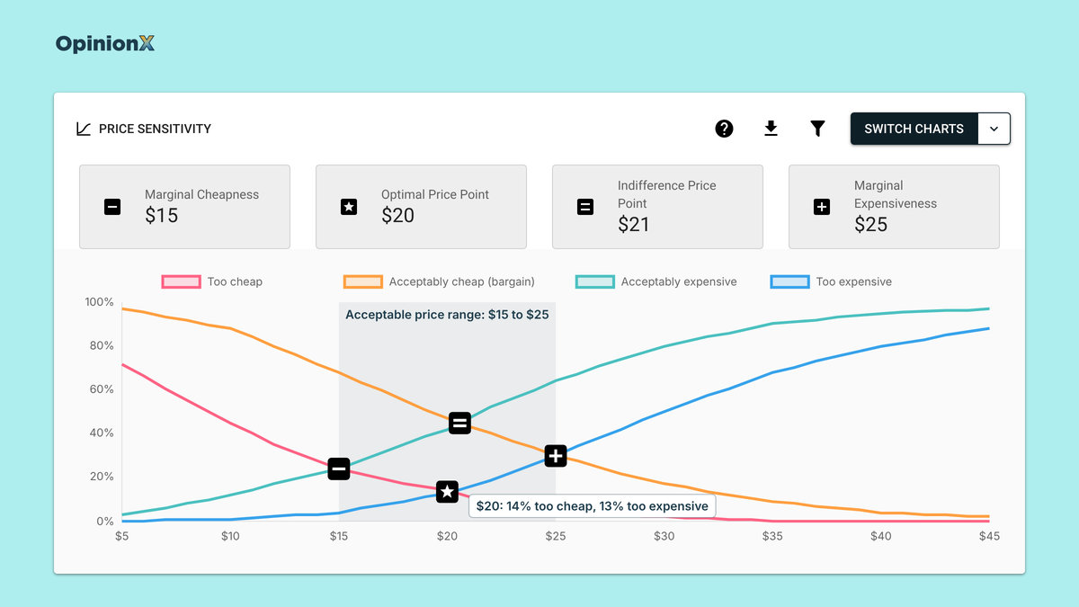
Each question turns into a line on a chart. The "too expensive" line shows the share of participants who said each price is too expensive, so it rises as the price goes up, and the "too cheap" line shows the share who'd doubt the quality at each price, so it falls as the price goes up. The price where those two lines cross is the optimal price point: the price the fewest participants reject outright, either as suspiciously cheap or as too expensive.
The optimal price point on its own isn't a price sensitivity measure, because it tells you where the middle is and not how strongly people react when you move away from it. Two other readings of the same chart do measure price sensitivity: the width of the acceptable price range and the steepness of the lines.
Reading price sensitivity from the acceptable price range
The acceptable price range sits between two more crossing points on the chart, and its width shows how tolerant participants are of different prices. The lower end, the point of marginal cheapness, is where the "too cheap" line crosses the "acceptably expensive" line. The upper end, the point of marginal expensiveness, is where the "acceptably cheap" line crosses the "too expensive" line. More participants reject than accept any price outside that range.
A narrow acceptable price range means high price sensitivity, because participants reject anything outside a small band of prices, while a wide one means low price sensitivity, because they'll consider lots of different prices.
Compare widths as a percentage of the price, not in dollars: an $8 range around a $14 price is much wider, relatively, than a $10 range around a $30 price. To get that percentage, divide the width by the midpoint of the range. In the Van Westendorp study on a 30oz Stanley Cup from our segmentation guide, with 134 participants, the acceptable price range was $15 to $25. That's $10 wide around a $20 midpoint, so 10 ÷ 20 = 50%.
Reading price sensitivity from the steepness of the lines
The steepness of the "too cheap" and "too expensive" lines either side of the optimal price point shows which direction of price change participants react to more. A "too cheap" line that climbs fast as you lower the price means participants are sensitive to price cuts, because a cheaper price makes them doubt the quality, while a "too expensive" line that climbs fast as you raise the price means they're sensitive to price rises.
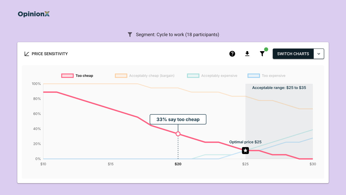
To measure this, read two shares off the chart: the share of participants calling the product too cheap at a fixed amount below the optimal price, and the share calling it too expensive at the same amount above it. In the Stanley Cup study, the cyclists' optimal price was $25, and at $20, just $5 below that, 33% of cyclists already said the cup was so cheap they'd doubt its quality. That group's price sensitivity points downwards: discounting the cup would cost you more cyclists than a price rise would, which a team looking only at the optimal price would've missed.
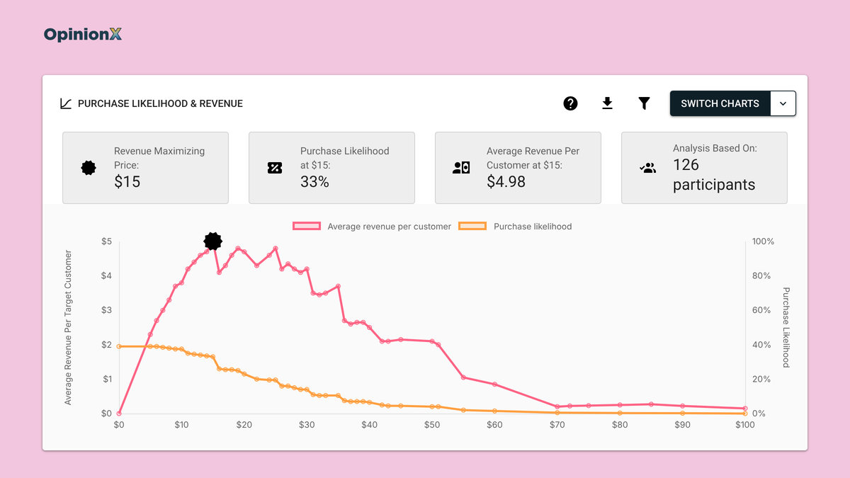
Van Westendorp has one big gap as a price sensitivity method: it measures how prices feel, not whether people would buy the product at those prices. Two extra questions, called the Newton-Miller-Smith (NMS) extension, ask Van Westendorp participants how likely they'd be to buy the product at the prices they gave for "bargain" and "getting expensive".
Their answers add a purchase likelihood figure you can use to project average revenue per customer at each price point. Our guide on the Newton-Miller-Smith extension shows how that calculation works, and our guide on how to read a Van Westendorp chart explains every crossing point with worked examples.
How does Gabor Granger measure price sensitivity?
Gabor Granger measures price sensitivity by asking each participant whether they'd buy a product at one specific price, then raising or lowering the price based on each answer until it finds the highest price that participant would pay.
Economists André Gabor and Clive Granger first published the method in the 1960s (ESOMAR, 1966), hence the name. Gabor Granger surveys add up every participant's highest accepted price to produce a demand line that shows the share of participants who'd buy the product at each price point.
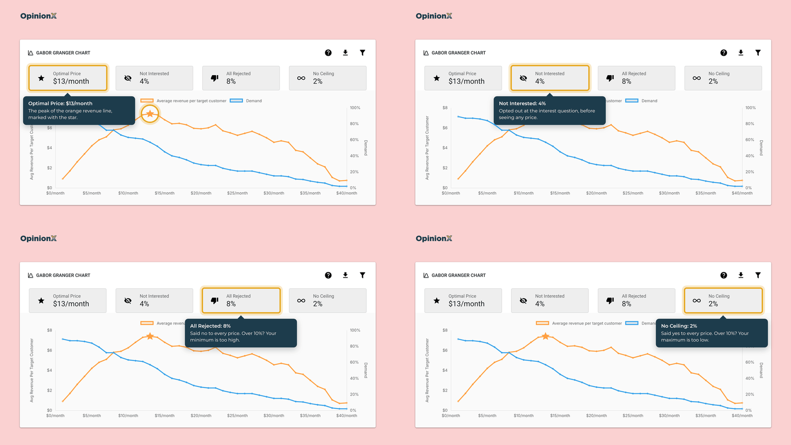
The demand line is a direct measure of price sensitivity, because it shows how buyer behaviour changes as the price rises, and you can calculate price elasticity from any two points on it. In the demo below, the slope of the blue "demand" line shows elasticity: the steeper the line falls, the more sensitive customers are to changes in that price range.
How do you calculate price elasticity from Gabor Granger results?
You calculate price elasticity between two neighbouring prices by dividing the percentage change in demand by the percentage change in price. Use the midpoint of each pair as the base for both percentages, so you get the same answer whether you move the price up or down.
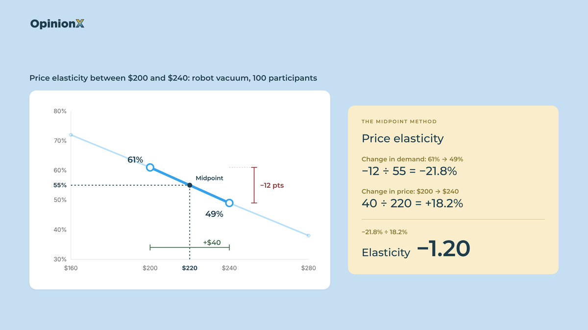
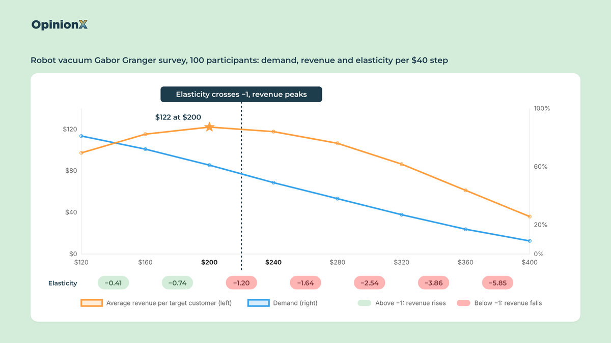
Here's a worked example using a Gabor Granger survey on a robot vacuum, with 100 participants voting on eight prices from $120 to $400 (the same dataset as our guide on Gabor Granger analysis). Take the step from $200 to $240:
Demand falls from 61% to 49%, a drop of 12 points around a midpoint of 55%, so the change in demand is −12 ÷ 55 = −21.8%.
Price rises from $200 to $240, a rise of $40 around a midpoint of $220, so the change in price is 40 ÷ 220 = +18.2%.
Price elasticity is −21.8% ÷ 18.2% = −1.20.
Do the same calculation for every pair of prices and you'll see the robot vacuum's price sensitivity change along the price range:
| Price step | Demand | Price elasticity | Average revenue per target customer |
|---|---|---|---|
| $120 → $160 | 81% → 72% | −0.41 | $97.20 → $115.20 🟢 |
| $160 → $200 | 72% → 61% | −0.74 | $115.20 → $122.00 🟢 |
| $200 → $240 | 61% → 49% | −1.20 | $122.00 → $117.60 🔴 |
| $240 → $280 | 49% → 38% | −1.64 | $117.60 → $106.40 🔴 |
| $280 → $320 | 38% → 27% | −2.54 | $106.40 → $86.40 🔴 |
| $320 → $360 | 27% → 17% | −3.86 | $86.40 → $61.20 🔴 |
| $360 → $400 | 17% → 9% | −5.85 | $61.20 → $36.00 🔴 |
While price elasticity sits between 0 and −1, customers are price insensitive in economic terms: a price rise loses a smaller share of buyers than the share it adds to the price, so revenue goes up. Once elasticity passes −1, every price rise loses a bigger share of buyers than it adds in price, and revenue goes down. So the revenue-maximising price in any Gabor Granger survey sits where elasticity crosses −1, which for the robot vacuum happens between $200 and $240, with the revenue line peaking at $200. The rest of the table tells you how quickly you'd lose revenue if you priced above it.
For context on what "normal" looks like, Gerard Tellis's analysis of 367 price elasticity estimates from more than 220 brands and markets found an average of −1.76 (Marketing Science Institute, 1988). Treat that as a rough reference point rather than a benchmark though, because those estimates came from actual sales data while survey elasticities come from stated answers.
Why the price range decides your Gabor Granger result
Gabor Granger only measures price sensitivity across the prices you choose to test, so a range that's too narrow or too low gives you a misleading demand line. Say the robot vacuum survey had stopped at $200: the revenue line would still be rising at the top of the range and the elasticity would never cross −1, so the result would tell you nothing about where demand starts to collapse. On OpinionX, two boxes on the results dashboard warn you about this, with "No Ceiling" counting participants who said yes to every price and "All Rejected" counting participants who said no to every price. If either box goes over 10% of participants, your price range needs to move. Our guide to choosing Gabor Granger price points shows how to set the minimum price, the number of prices and the interval (the gap between each price) so the range covers the actual answer.
Choosing the price range is the step most first-time pricing surveys get wrong, and it's hard to fix once participants have answered. If you'd like a second pair of eyes on your price range before you launch, book a free 30-minute setup call and a research expert will check your prices, interval and sample size.
How does a conjoint survey measure price sensitivity?
A conjoint analysis survey measures price sensitivity by showing participants sets of product versions that mix features and prices, and asking them to pick the one they'd choose. Participants have to trade price against features in every choice, so conjoint analysis shows price sensitivity in context, which Van Westendorp and Gabor Granger can't, since they price the product on its own.
Price is one category in a conjoint survey, alongside the product's other features. A category is one feature you're testing, like storage, and its options are the values it can take, like 128GB or 256GB. From each participant's choices, conjoint analysis works out a score for every option, meaning how much that option raises or lowers the chance the participant picks a product version. OpinionX calculates those scores for each participant with a Hierarchical Bayes model, a statistical model that estimates scores person by person instead of only for the group as a whole.
The four conjoint sections below all use the same dataset: a smartphone conjoint survey that 1,363 people completed on OpinionX as our public demo survey. Each participant chose between phones that combined three categories:
Brand: iPhone, Samsung, Google Pixel or Huawei
Memory: 128GB, 256GB, 512GB or 1TB
Price: $419, $659 or $899
The survey also asked which operating system each participant's current phone uses (770 said iOS and 529 said Android), which is what makes the segment comparison later in this guide possible. The participants are people who tried our demo, not a recruited sample of phone buyers, so treat the results as a worked example of each method and not as a market study of smartphones.
How does price importance measure price sensitivity?
Price importance measures price sensitivity as the share of participants' decisions driven by price rather than by the product's features. It's the first figure most conjoint results show, and the calculation has three steps:
For each category, subtract the lowest option score from the highest option score. That difference is the category's range.
Add up the ranges of every category.
Divide the price category's range by the total.
Here's that calculation on the smartphone survey's overall scores, which OpinionX shows as percentages:
| Category | Highest-scoring option | Lowest-scoring option | Range | Importance |
|---|---|---|---|---|
| Brand | iPhone, +6.41 | Huawei, −6.5 | 12.91 | 48.5% |
| Memory | 1TB, +3.57 | 128GB, −3.8 | 7.37 | 27.7% |
| Price | $419, +3.12 | $899, −3.22 | 6.34 | 23.8% |
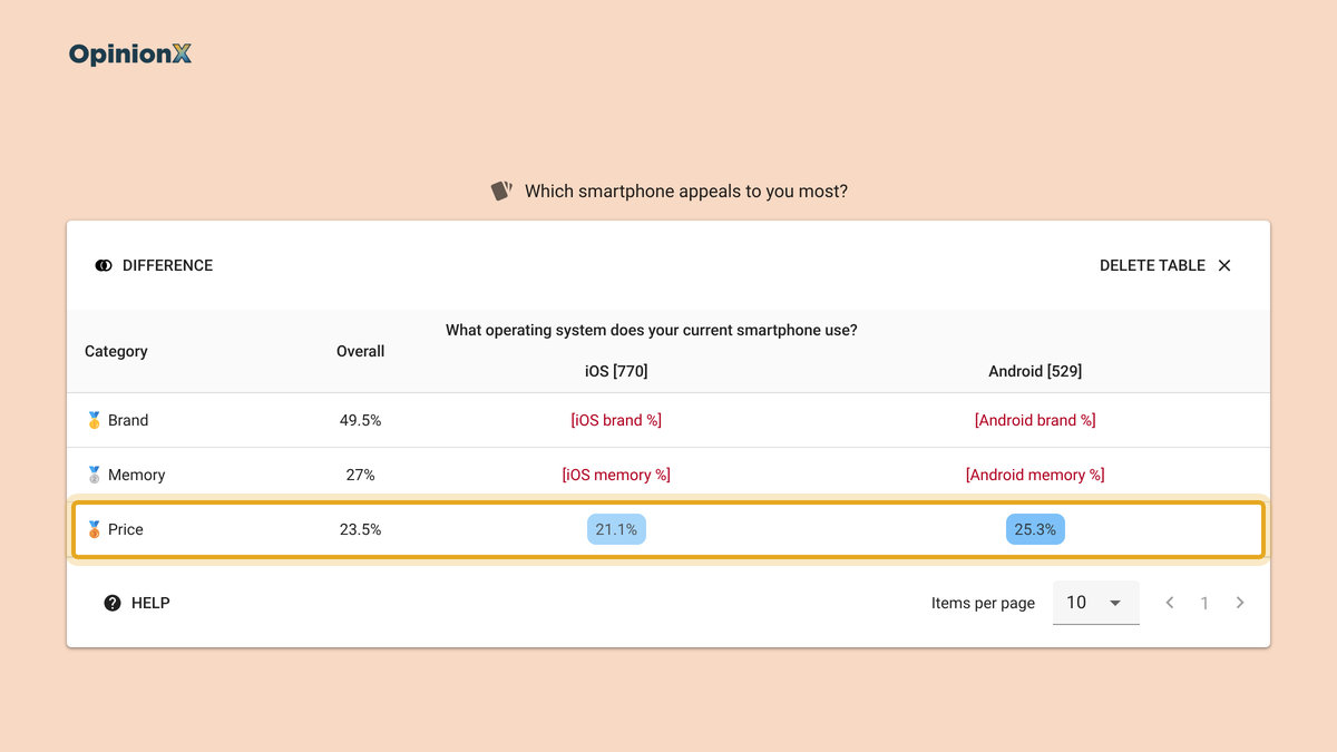
The total range is 12.91 + 7.37 + 6.34 = 26.62, so price importance is 6.34 ÷ 26.62 = 23.8%. OpinionX's results dashboard shows 23.5% for price, slightly lower, because it does the same calculation for each participant and then averages the results, which is the more accurate way to do it. Either way, price drove just under a quarter of participants' choices, memory just over a quarter and brand about half.
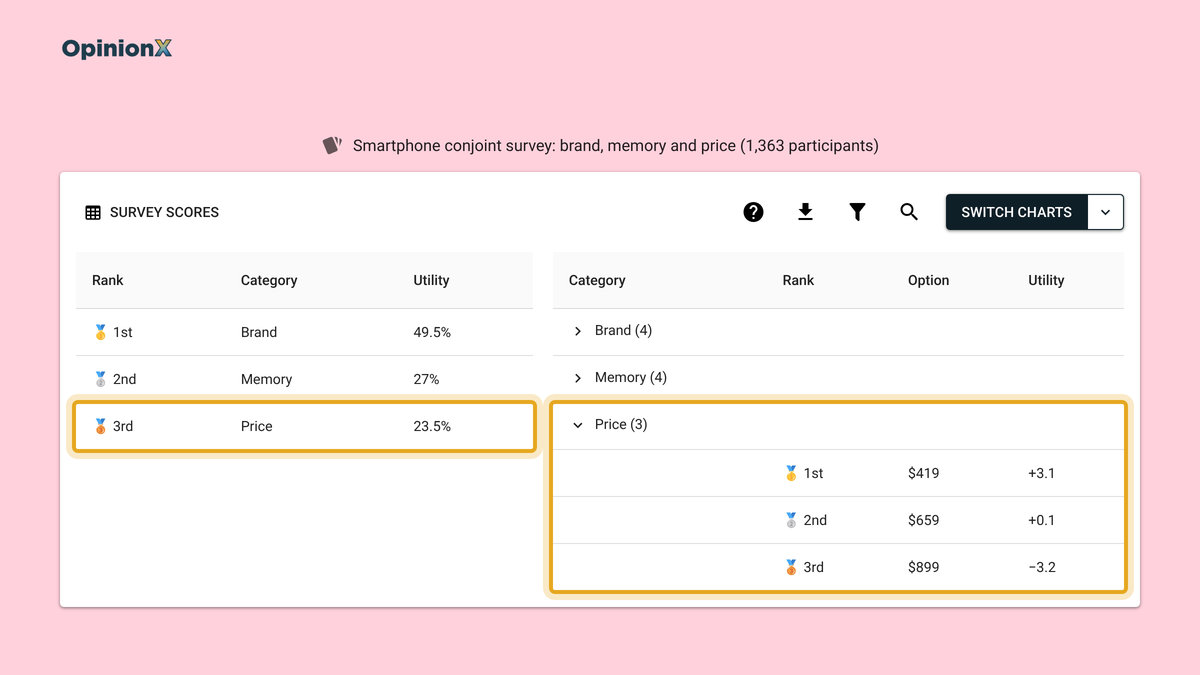
Price importance is a relative measure, so it changes with the options you test. If the smartphone survey had tested prices from $419 to $1,299 instead of $419 to $899, price importance would go up, because a wider spread of prices gives price more weight in each choice. That makes price importance useful for comparing customer segments, or two studies with the same design, but not as a stand-alone figure. "23.5%" on its own doesn't tell you whether to raise prices, while Android owners at 25.3% against iPhone owners at 21.1% tells you which group a price rise would lose first. Our guide on how to calculate conjoint analysis results walks through the full calculation step by step.
How does marginal willingness to pay measure price sensitivity?
Marginal willingness to pay (MWTP) measures price sensitivity in dollars, by calculating how much extra customers would pay to upgrade one feature of a product. It comes from any conjoint survey with a price category, so you don't need to ask participants any extra questions.
The MWTP calculation turns conjoint scores into money in two steps. First it works out how many dollars of price equal one point of score, by fitting a straight line through the price options and their scores. In the smartphone survey, the price score falls from +3.12 at $419 to −3.22 at $899, a drop of 6.34 points across $480 of price, so one point of score is worth $480 ÷ 6.34 = $75.71. Then it multiplies the score gap between two options by that dollar value:
| Upgrade | Score gap | Marginal willingness to pay |
|---|---|---|
| 128GB → 256GB | 2.84 | $215 |
| 256GB → 512GB | 2.16 | $164 |
| 512GB → 1TB | 2.37 | $179 |
| Google Pixel → Samsung | 0.67 | $51 |
| Samsung → iPhone | 6.05 | $458 |
MWTP is the price sensitivity measure that roadmap and tier decisions need. The table says the first memory upgrade, from 128GB to 256GB, is worth the most to participants at $215, and each later upgrade is worth less, the usual pattern for a feature people need a minimum amount of. If the 256GB to 512GB upgrade costs you less than $164 to provide, it can sit in a higher tier or a paid add-on. The brand rows go further: participants would pay $458 more for an iPhone than for an otherwise identical Samsung, which is more than the whole $480 price range the survey tested.
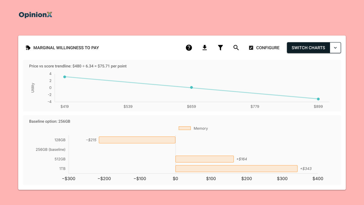
The Marginal Willingness To Pay report on OpinionX draws the price line and the bars for you, and lets you click any bar to change the baseline option, so you can value every upgrade against the version you sell today. Our guide to marginal willingness to pay walks through the automatic report and a Google Sheets version for doing it by hand, including what to do when the price line curves.
MWTP has two limits. First, it only values the gap between two options, never a feature on its own and never the whole product, because every score in conjoint is relative to the other options. Second, it inherits conjoint's overstatement: a meta-analysis by Schmidt and Bijmolt found that indirect methods like conjoint overstate willingness to pay by about 10 percentage points more than direct questions do (Journal of the Academy of Marketing Science, 2020). Use MWTP to rank upgrades against each other and treat the dollar figures as an upper estimate; a $458 brand premium that's bigger than the tested price range is a sign to read it that way.
How does rejection rate measure price sensitivity?
Rejection rate measures price sensitivity by counting how often conjoint participants pick "None of the above" instead of a product version, split by each option, including each price.
A standard conjoint survey uses forced choice, meaning participants have to pick one of the product versions shown even if they wouldn't buy any of them. Forced choice is good at showing which version people prefer, but it can't show whether they'd buy at all, because a price rise only moves participants from one version to another and never out of the market. Actual customers can also buy nothing. Adding a "None of the above" button to each set of product versions gives participants that choice, so a price that's too high for them shows up as a rejection instead of a reluctant vote. Our guide to forced choice questions explains when forcing a choice helps a survey and when it hides the answer you need.
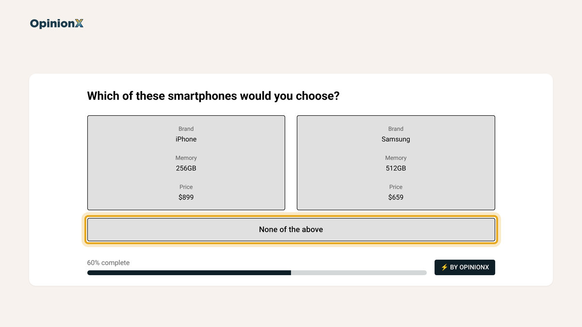
The rejection rate for an option is the number of times participants picked "None of the above" divided by the number of voting sets in which that option appeared on at least one product version. If the $899 option appeared in 1,000 voting sets and participants picked "None of the above" in 150 of them, the $899 rejection rate is 150 ÷ 1,000 = 15%.
The smartphone survey collected its votes without the "None of the above" button switched on, so the rates in this paragraph are an illustration and not survey data. Say the $419 option has a 4% rejection rate, $659 has 7% and $899 has 15%. The jump between $659 and $899 is where price turns from a trade-off into a reason not to buy, which price importance can't tell you, since it only shows how much price drives the choice between versions and not how many people would leave the market at a given price. Compare the price options' rejection rates with the feature options' rates too, to see whether a weak option, like a 128GB phone, drives more rejections than any price does.
The wording of the "None of the above" button decides what the rejection rate means, so write it for your decision. On OpinionX the button text is customisable: a survey for current customers could label it "Stay on the current plan", which makes the rejection rate a measure of how many would refuse to upgrade, while a survey for new prospects could say "None of these". The None of the above release notes show the Rejection Rate chart and the button settings, and rejection counts also appear in the Segments Tab and survey exports, so you can compare rejection rates between customer segments.
Rejection Rate has two catches. You have to turn on the "None of the above" option before launch, because you can't add it once participants have voted. The rejection rate also depends on how often each option appears, so an option shown in only a few voting sets gives an unstable rate. Check that every price option appears often enough, which for most studies comes from having enough participants rather than from changing the design.
How does a revenue simulator measure price sensitivity?
A revenue simulator measures price sensitivity by predicting how market share and revenue change when you change the price of one product version while others stay on offer. On OpinionX, the Scenario Simulator on every conjoint results dashboard has three modes: market share, revenue and churn.
The simulator works person by person. You build two or more product versions by picking one option from each category, and for every participant, the simulator uses that person's own conjoint scores to predict which version they'd pick, then adds up those predictions into market shares that total 100%. Revenue is each version's price × its market share × a fixed base of 1,000 customers.
Here's what it shows on the smartphone survey, with a 256GB Samsung repriced at each of the three tested prices against a 256GB Google Pixel that stays at $659:
| Samsung price | Samsung market share | Samsung revenue (per 1,000 customers) | Price elasticity from the previous price |
|---|---|---|---|
| $419 | 87% | $364,530 | n/a |
| $659 | 61% | $401,990 🟢 | −0.79 |
| $899 | 20% | $179,800 🔴 | −3.29 |
The elasticity column uses the same midpoint method as the Gabor Granger section. From $419 to $659, market share falls 26 points around a midpoint of 74%, a change of −35.1%, while price rises $240 around a midpoint of $539, a change of +44.5%. Elasticity is −35.1% ÷ 44.5% = −0.79, so the price rise loses a smaller share of buyers than it adds in price and revenue goes up. From $659 to $899, elasticity is −3.29 and revenue falls by more than half. The Samsung earns the most at $659, the same price as the Pixel, and the drop above that price is far steeper than the drop below it.
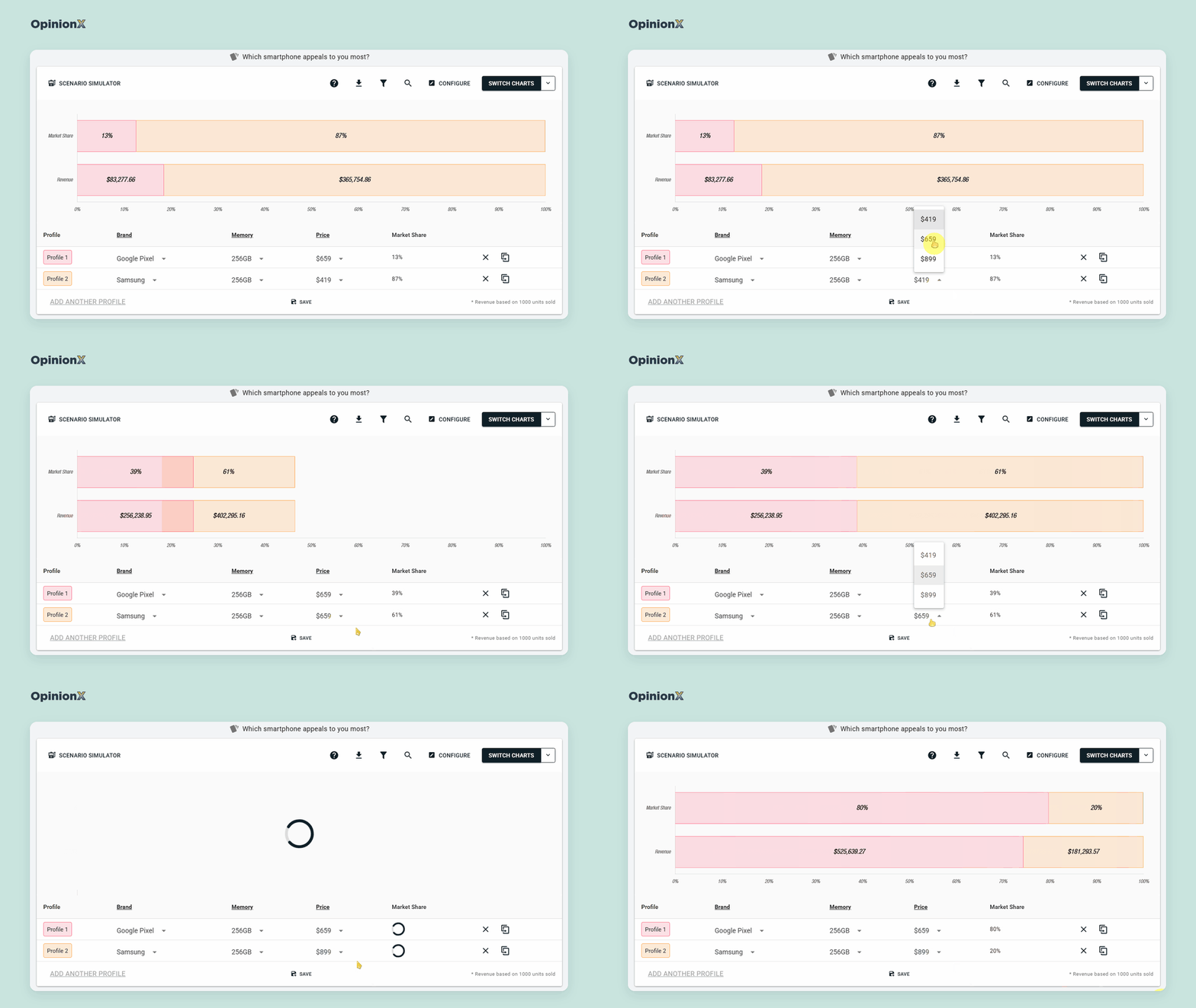
The revenue simulator measures price sensitivity in a way Gabor Granger can't, because the price change happens while a competing version stays on the table. A Gabor Granger participant only decides whether to buy one product at one price, while a simulated participant can switch to the Pixel or, with the churn mode and a "None of the above" option in the survey, to buying nothing. Without that option, every participant always picks one of your versions, which can make high prices look less costly than they are. Our guide to the conjoint market simulator shows how to build pricing scenarios with more than two versions.
The revenue simulator has three limits:
The 1,000 customers is a fixed base, so read revenue as a comparison between scenarios, not as a forecast of your actual sales.
Market share is shared only among the versions you build, so leaving out an actual alternative (like an iPhone in this example) makes your versions look stronger than they'd be in the market.
Like every conjoint output, the simulator inherits the overstatement in stated willingness to pay, so it's best at telling you which of two prices earns more, not exactly how much.
Want to see a Scenario Simulator reprice a product version live, alongside the price importance, MWTP and Rejection Rate charts? A demo walks through all four on one conjoint results dashboard.
How do you compare price sensitivity across customer segments?
You compare price sensitivity across customer segments by asking participants a few questions about themselves in the same survey, then filtering the pricing results to one group at a time. A customer segment is any group you want to look at on its own, such as job role, company size, current plan or how people use the product. Segment comparison is where price sensitivity research turns into a decision, because it shows which customers to price for, which to discount for and which to leave alone.
The Stanley Cup study shows why. Across all 134 participants, the acceptable price range was $15 to $25 and the optimal price was $20, but filtering by how participants get to work told a different story:
| Segment | Participants | Acceptable price range | Optimal price | Range width ÷ midpoint |
|---|---|---|---|---|
| Everyone | 134 | $15 to $25 | $20 | 50% |
| Cycle to work | 18 | $25 to $35 | $25 | 33% |
| Drive | 34 | $19 to $30 | $20 | 45% |
| Don't commute | 23 | $15 to $25 | $20 | 50% |
| Walk | 25 | $13 to $25 | $15 | 63% |
| Public transport | 24 | $10 to $18 | $10 | 57% |
The cyclists and the public transport users have acceptable price ranges that don't overlap at all, so the $20 price that looked right for everyone sits outside the acceptable price range of both groups. The range width column adds a second finding: cyclists would pay the most, but their acceptable price range is the narrowest relative to the price, at 33%, so they're the least tolerant of a price that's off in either direction, while walkers would pay less but have the widest range, at 63%, so a price a little above their optimal price costs fewer of them.
Put the optimal price and the range width together and segments sort into four types of buyer:
| Low optimal price | High optimal price | |
|---|---|---|
| Narrow range | 🏷️ Bargain hunters: price them low and avoid price rises | 💎 Premium but demanding: price them high and avoid discounts (the cyclists) |
| Wide range | 🧺 Value-focused but flexible: room to test small price rises (the walkers) | 🛋️ Least price sensitive: the best candidates for a premium tier |
Don't be fooled by small segments though. The cyclist group had only 18 participants, so its optimal price is a rough reading. When the Stanley Cup study resampled each group's answers 2,000 times, the cyclists' optimal price landed anywhere between $15 and $40 in 90% of the samples, and it still came out higher than the public transport group's in 97% of them.
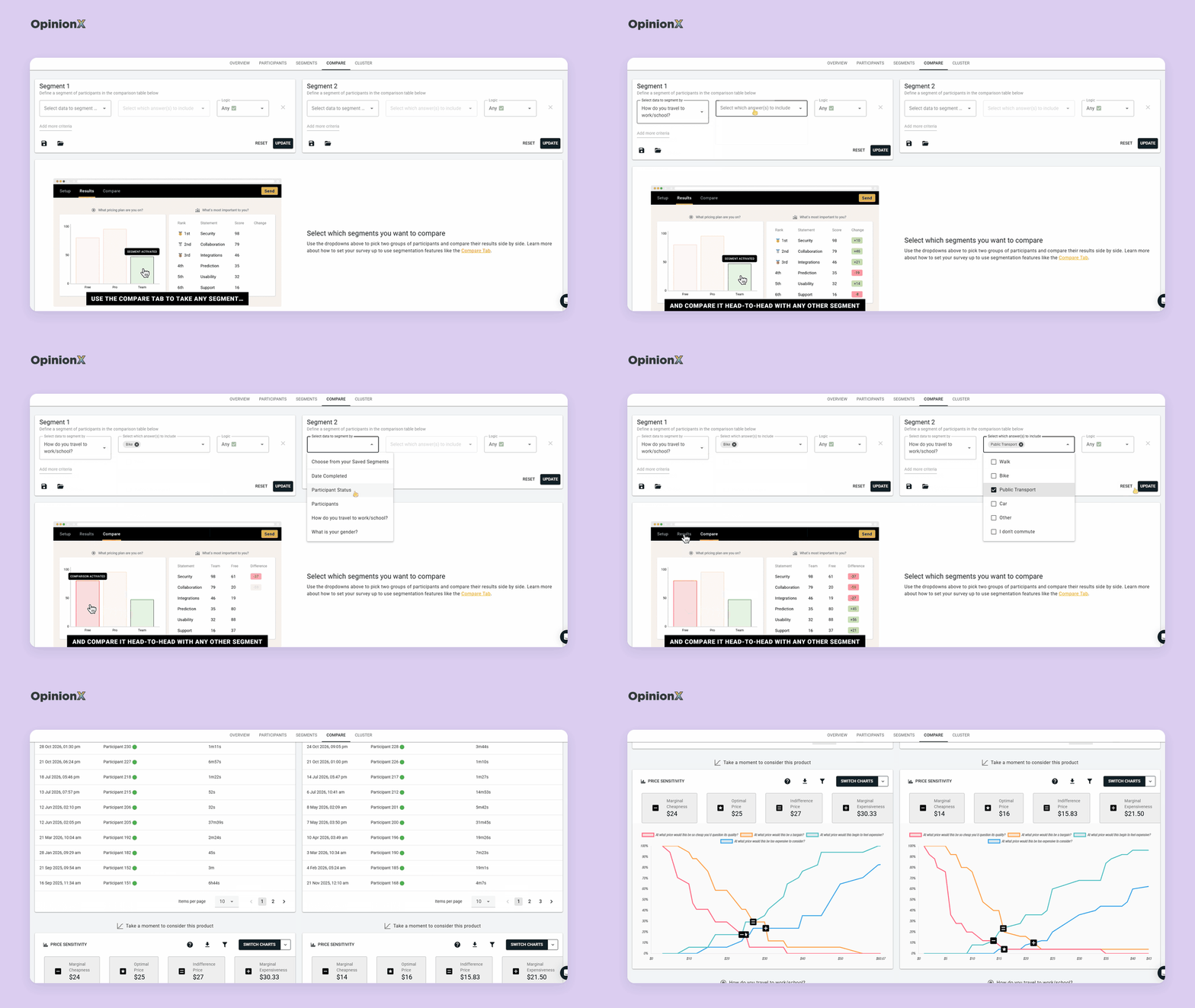
Our guide on Van Westendorp segmentation explains that check in full, and our Van Westendorp sample size calculator shows how many participants each segment needs. If you're recruiting participants yourself without a paid panel, our guide to finding free survey participants covers three ways to do it.
How do conjoint results compare price sensitivity between segments?
Conjoint results compare price sensitivity between segments the same way: filter the results to one group, and all four conjoint readings recalculate for that group. In the smartphone survey, splitting participants by the operating system on their current phone shows two groups with very different price sensitivity:
| Segment | Participants | Price importance | Dollars per point of score | Extra they'd pay for an iPhone over a Samsung |
|---|---|---|---|---|
| Everyone | 1,363 | 23.5% | $75.71 | $458 |
| Current phone runs iOS | 770 | 21.1% | $89.22 | $711 |
| Current phone runs Android | 529 | 25.3% | $63.66 | $208 |
All three columns point the same way. Android owners give price more weight in their choices, at 25.3% against 21.1%, and each point of score is worth fewer dollars to them, at $63.66 against $89.22, because their price score falls more steeply (from +3.70 at $419 to −3.84 at $899, against +2.65 to −2.73 for iPhone owners). The brand premium splits completely too: iPhone owners would pay $711 more for an iPhone than an otherwise identical Samsung, while Android owners would pay $208 more. The overall $458 describes neither group, which is the same lesson as the Stanley Cup segments, reached with a different survey.
How do you collect customer segmentation data in a pricing survey?
You collect segment data by adding multiple-choice questions to your pricing survey, such as "What's your role?" or "How many people work at your company?". Each answer tags the participant, so you can filter the pricing results by that group afterwards. If you already hold data about your customers, you can skip some of those questions: hidden fields pass details like plan or account size through the survey link, and participant data enrichment lets you import columns from your CRM after the survey closes.
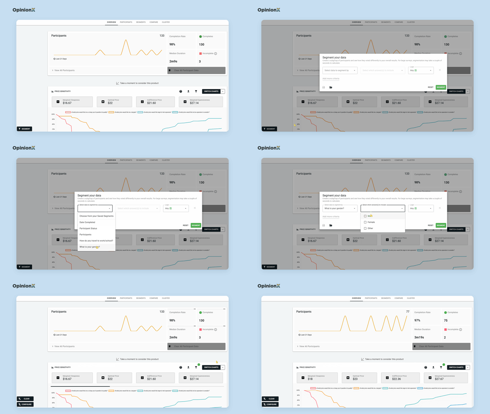
Pick segments that match a decision you could actually make, like "Current plan" (Free, Pro, Enterprise), which maps straight onto a pricing tier decision. Our guide to needs-based segmentation explains how to group customers by what they're trying to get done, which often splits price sensitivity more sharply than job title does. The segmentation features on OpinionX recalculate every chart for one group with a single filter, and a crosstab (a table with one column per segment) shows every group's result side by side. For Gabor Granger, our guide on how to segment Gabor Granger results applies the same process to a demand line.
Want to see a pricing chart recalculate for each customer segment before you build your own study? A demo walks through actual Van Westendorp, Gabor Granger and conjoint results, filters, Segments Tab and all.
What are the common mistakes when measuring price sensitivity?
Most price sensitivity studies that fail go wrong in how someone set them up or read the results, not because of the method, and four mistakes come up again and again.
The first mistake is reading survey answers as actual spending. People say in surveys that they'd pay about 21% more than they really do when money is on the line, according to a review of 77 studies by Schmidt and Bijmolt (Journal of the Academy of Marketing Science, 2020). That gap doesn't make pricing surveys useless though. Klaus Miller and his co-authors tested four ways of measuring willingness to pay against actual purchases and concluded that methods with this bias "may still lead to the right demand curves and right pricing decisions" (Journal of Marketing Research, 2011). Surveys get the relative picture right more reliably than the exact prices, so trust where the revenue peak sits and which segment is more price sensitive, and treat any revenue figure as an upper estimate.
The second mistake is measuring price sensitivity without knowing where prices sit. A segment can be very price sensitive around $10 or around $100, and the two mean completely different businesses. Conjoint price importance on its own tells you how much weight price carries, not what price to charge, so pair it with a Van Westendorp or Gabor Granger question in the same survey and you'll get both how sensitive each segment is and where its prices sit. Our guide to running Van Westendorp and Gabor Granger in one survey shows how to set that up.
The third mistake is forgetting to plan for segmentation. If you don’t have a way to enrich your results with existing data or your survey doesn't ask who participants are, you can't split the results later, and you're stuck with one average price for a mix of very different customers. Add the multiple-choice questions before launch, because you can't add them after people have answered. The same goes for the "None of the above" option in a conjoint survey, which rejection rate and the simulator's churn mode both depend on.
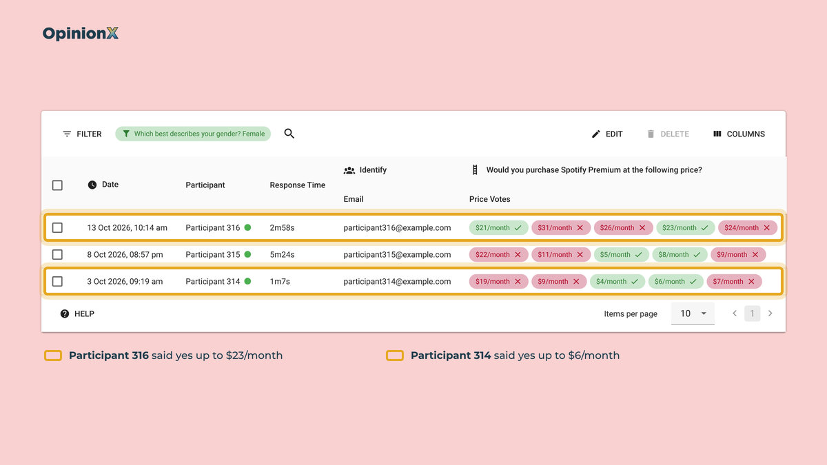
The fourth mistake is running the survey anonymously. A pricing survey shows you what participants would pay, not why. Collect participants' email addresses (with their permission) and you can invite the most and least price sensitive participants to a short follow-up interview to ask what drives their answers. The Discovery Sandwich is our three-layer product discovery framework built on this idea: broad interviews to find customers' problems, then a survey to rank those problems, then focused interviews on what the survey picked out. Our guide to participant-level data shows how to find the individual participants who represent each segment.
What are the limitations of measuring price sensitivity with a survey?
A pricing survey can't tell you how customers will react to competitors' prices unless you put those competitors in the survey, because Van Westendorp and Gabor Granger both price your product on its own. If customers compare you head-to-head with a named alternative, a conjoint survey that includes competitor versions, read through a revenue simulator, gets closer to the choice they actually face.
Surveys can't replace behaviour either, because price sensitivity measured in a survey is what people say before they've paid. Once you've launched a price, actual sales data, churn after a price change and A/B tests on a pricing page are better evidence than any survey, and the survey's job shifts to explaining why sales moved and which segments moved them. Our guide to A/B testing with surveys covers how to test price messaging when you don't have enough traffic for a live experiment.
Finally, you only measure price sensitivity for the product you describe, so a vague description gets you a vague answer. Give participants the price unit and billing period ("per month, per user") and the main features, because participants who picture different products answer different questions, and you can't spot or fix that in the data afterwards.
Frequently asked questions
What does a price elasticity of −1 mean? A price elasticity of −1 means a 10% price rise cuts demand by exactly 10%, so revenue stays the same. Above −1, such as −0.5, a price rise increases revenue, while below −1, such as −2, a price rise loses revenue. The revenue-maximising price sits where elasticity crosses −1.
How many participants does a price sensitivity survey need? A price sensitivity survey needs about 100 participants for a rough answer. Mike Pritchard of 5 Circles Research recommends at least 200 participants for business products and 400 for consumer products. To compare customer segments, each segment needs about 100 participants of its own.
What's the difference between price sensitivity and willingness to pay? Willingness to pay is the highest price one customer would pay for a product, while price sensitivity is how much demand changes as the price changes, across many customers. Willingness to pay tells you where a price sits, and price sensitivity tells you how many buyers a move away from that price would cost you.
What is a rejection rate in conjoint analysis? A rejection rate in conjoint analysis is how often participants picked "None of the above" when a product version containing a specific option was on screen. A rejection rate that jumps at one price option shows where price stops being a trade-off and becomes a reason not to buy at all.
Which method is best for measuring price sensitivity? The best method depends on the pricing decision. Van Westendorp suits a product with no price yet, and Gabor Granger finds the revenue-maximising price for one product. A conjoint survey suits decisions about features, tiers and competitors, through price importance, marginal willingness to pay, rejection rate and a revenue simulator.
If you're pricing a single product and don't have a price yet, start with our Van Westendorp pricing guide, which covers the four questions, the chart and how OpenAI priced ChatGPT's $20 plan. If you already have a rough price range, our Gabor Granger method guide explains how the price search works and how to set it up. If you're pricing features, tiers or competing product versions, our conjoint analysis guide covers how to design the survey, and our guide on when not to use conjoint analysis covers the cases where a simpler method gives a better answer. Our comparisons of Van Westendorp vs Gabor Granger and Van Westendorp vs conjoint analysis help if you're choosing between two of them. Still deciding which features to include before you price them? Our guide to MaxDiff analysis shows how to rank features by importance.
Every pricing method on OpinionX, including Van Westendorp, Gabor Granger and conjoint analysis with all four conjoint reports, is on our free plan for up to 25 participants per survey. The Analyze plan removes the participant limit for $900 per year, with unlimited researcher seats (see pricing).
